Lattice learning 2

这篇博客refer的东西太多了，所以要看别的师傅的版本的话可以转路友链里的密码师傅们

Preface

格子真是好玩的东西，但是看得再多的博客也不如自己亲自调几个格子来的清楚，比如各种优化或者约束

Chapher 5 Encryption mode in Lattice

Coppersmith

Coppersmith是啥？

铜匠！炼铜！

在我看来就是一种在有限域内解方程的方法，比方说 $f(x)=x^4+114x+514$ 且对于有特殊关系的 $x_0$ 满足关系 $f(x_0)\equiv0\pmod{N}$ ，去求解这样的 $x_0$ 时我们可以使用Coppersmith’s methed。对于度为 $d$ 的多项式 $f(x)$ ，如果这个 $x_0$ 满足 $|x0|< N^{\frac{1}{d}-\varepsilon}$ ，那么就能在多项式的时间内被找出。

假设 $N$ 是一个未知因子组成的数，且存在一个因子 $b\geq N^\beta(0<\beta\leq 1)$ ，$f(x)$ 是一个一元一次 $d$ 阶的多项式，且 $c\geq 1$ ，那么可以在 $O(cd^5log^9(N))$ 的复杂度内求解所有的 $x_0$ 。

$f(x_0)=0\pmod{b},x_0\leq cN^{\frac{\beta^2}{d}}$

这里关于证明，等我有时间把高等代数学会了再回来证

线性代数中我们学过：任何的函数都可以被写成一个基函数的样子，当然求导也是一种线性变换，如下图：
$$
Basis~functions{=\begin{bmatrix}
1\\x\\x^2\\x^3\\\vdots
\end{bmatrix}}
~~
\frac{d}{dx}=
{\begin{bmatrix}
0&1&0&0&\cdots\\
0&0&2&0&\cdots\\
0&0&0&3&\cdots\\
0&0&0&0&\cdots\\
\vdots&\vdots&\vdots&\vdots&\ddots
\end{bmatrix}}
$$
说了这么多，Coppersmith到底是干嘛的？对于一元Coppersmith，它的作用就是找出一个 $F(x)=A\cdot f(x)-N\cdot g(x)$ ，这样就能利用牛顿法求出使得 $F(x)=0$ 的 $x_0$ ，那么此时 $f(x_0)\equiv0$ 也是显而易见的了。

我们不妨把函数 $f(x)=x^d+a_{d-1}x^{d-1}+\cdots+a_1x+a_0$ 表示成一个类似基函数的向量： $\vec{a}=(a_0,xa_1,x^2a_2,\cdots,x^da_d)$ ，那么只要 $||\vec{a}||<\frac{N}{\sqrt{d+1}}$ 且 $F(x_0)\equiv0\pmod{N}$ ，就有 $f(x_0)\equiv0$ ，关于Coppersmith的证明和界的扩大方法这里指路V神的博客。

已知部分明文攻击

设 $m=m_0+x$ ，我们可以找到 $f(x)=(m_0+x)^e-c\pmod{N}$ ，当 $e$ 和 $x$ 较小时，Coppersmith即可计算出 $x$ 的值

$b=N,d=e,\beta=1$ 则 $|x|\leq cN^{\frac{\beta^2}{d}}=cN^{\frac{1}{e}}$ ，因此为了求解，我们至少需要知道关于m至少 $(1-\frac{1}{e})\cdot N.bit_length()$ bit的信息

e = 
c = 
n = 
kbits = # unknow x bit
m0 = 
PR.<x> = PolynomialRing(Zmod(n))
f = # f(x)
f = f.monic()
x0 = f.small_roots(X=2^kbits,beta=1)[0]
print(x0)

已知部分因子攻击

设 $p=p_0+x$ ， $f(x)=p_0+x$ 此时我们把 $N$ 看做 $k\cdot p$ ，又因为 $-p_0\equiv x\pmod{p}$ ，则可以找到 $K\cdot f(x)-M\cdot p=0$

$b=p$ ，且RSA中 $p$ 和 $q$ 通常是满足 $p<q<2p$ 所以 $p\approx N^{0.4}$ ，也就是说 $\beta=0.4$ 附近较为适合，另外 $|x|<N^{\frac{1}{3}}$ ，我们只要知道 $p$ 一半bit就可以求出这样的 $x$ 。

n = 
p0 = 
kbits = 
PR.<x> = PolynomialRing(Zmod(n))
f = # f(x)
# f = f.monic()
x0 = f.small_roots(X=2^kbits, beta=0.4)[0]
p = x0 + p0
print(p)

已知部分私钥攻击

来自论文《An Attack on RSA Given a Small Fraction of the Private Key Bits》

设 $d=d_0+x$ ，且 $d_0$ 是私钥 $d$ 的kbits低位，那么显然 $d_0\equiv d\pmod{2^{kbits}}$ ，那么有 $e\cdot d_0=e\cdot d=1+k\cdot\varphi(N)=1+k(N-(p+q)+1)\pmod{2^{kbits}}$ ，

则通过解方程 $e\cdot d_0\cdot X-k\cdot X\cdot(N-X+1)=X$ 就可以得到所有可能的 $i\cdot p+j\cdot q\pmod{2^{kbits}}$ 的值，接着再求解 $p^2-xp+N=0\pmod{2^{kbits}}$ 即可得到 $p$ 的低位值，将上面两个式子联立，即只需要解一个方程 $e\cdot d_0\cdot X - k\cdot X\cdot(n-X+1) + k\cdot n == X$ 即可得到低位的 $p$

def partial_p(p0, kbits, n):
    PR.<x> = PolynomialRing(Zmod(n))
    nbits = n.nbits()

    f = 2^kbits*x + p0
    f = f.monic()
    roots = f.small_roots(X=2^(nbits//2-kbits), beta=0.3)
    if roots:
        x0 = roots[0]
        p = gcd(2^kbits*x0 + p0, n)
        return ZZ(p)

def find_p(d0, kbits, e, n):
    X = var('X')

    for k in range(1, e+1):
        results = solve_mod([e*d0*X - k*X*(n-X+1) + k*n == X], 2^kbits)
        for x in results:
            p0 = ZZ(x[0])
            p = partial_p(p0, kbits, n)
            if p:
                return p

n = 
e = 
d = 
nbits = n.nbits()
kbits = d.nbits()

p = find_p(d, kbits, e, n)
q = n//p
print("p = %d" % p)
print("q = %d" % q)
print("d0 = %d" % d)
print("d = %d" % inverse_mod(e, (p-1)*(q-1)))

多消息攻击

线性相关消息攻击

已知 $c1=m^e\pmod{N}$ ， $c2=(a\cdot m+b)^e\pmod{N}$

首先用 $e=3$ 举个栗子，我们可以通过构造 $m=\frac{m\cdot f(m)}{f(m)}$ 的格式来求 $m$ ，比方说 $e=3$ 时，我们能构造 $m=\frac{b}{a}\cdot\frac{c_2+2a^3c_1-b^3}{c_2-a^3c_1+2b^3}$

关于更高维的，等我学会就来写，这里指路《Low-Exponent RSA with Related Messages》

多消息相关攻击

Waiting for undate……

Hastad广播攻击

Waiting for undate……

SMUPE攻击

Waiting for undate……

Boneh and Durfee attack

Waiting for undate……

先放一个别人的版本，等后面自己实现完了之后来换

#!python3
# -*- coding: utf-8 -*-
# @Time : 2020/10/31 23:37
# @Author : A.James
# @FileName: tt6.py
# @Email : alexjames@sina.com
import time

############################################
# Config
##########################################

"""
Setting debug to true will display more informations
about the lattice, the bounds, the vectors...
"""
debug = True

"""
Setting strict to true will stop the algorithm (and
return (-1, -1)) if we don't have a correct 
upperbound on the determinant. Note that this 
doesn't necesseraly mean that no solutions 
will be found since the theoretical upperbound is
usualy far away from actual results. That is why
you should probably use `strict = False`
"""
strict = False

"""
This is experimental, but has provided remarkable results
so far. It tries to reduce the lattice as much as it can
while keeping its efficiency. I see no reason not to use
this option, but if things don't work, you should try
disabling it
"""
helpful_only = True
dimension_min = 7  # stop removing if lattice reaches that dimension


############################################
# Functions
##########################################

# display stats on helpful vectors
def helpful_vectors(BB, modulus):
    nothelpful = 0
    for ii in range(BB.dimensions()[0]):
        if BB[ii, ii] >= modulus:
            nothelpful += 1

    print (nothelpful, "/", BB.dimensions()[0], " vectors are not helpful")


# display matrix picture with 0 and X
def matrix_overview(BB, bound):
    for ii in range(BB.dimensions()[0]):
        a = ('%02d ' % ii)
        for jj in range(BB.dimensions()[1]):
            a += '0' if BB[ii, jj] == 0 else 'X'
            if BB.dimensions()[0] < 60:
                a += ' '
        if BB[ii, ii] >= bound:
            a += '~'
        print (a)


# tries to remove unhelpful vectors
# we start at current = n-1 (last vector)
def remove_unhelpful(BB, monomials, bound, current):
    # end of our recursive function
    if current == -1 or BB.dimensions()[0] <= dimension_min:
        return BB

    # we start by checking from the end
    for ii in range(current, -1, -1):
        # if it is unhelpful:
        if BB[ii, ii] >= bound:
            affected_vectors = 0
            affected_vector_index = 0
            # let's check if it affects other vectors
            for jj in range(ii + 1, BB.dimensions()[0]):
                # if another vector is affected:
                # we increase the count
                if BB[jj, ii] != 0:
                    affected_vectors += 1
                    affected_vector_index = jj

            # level:0
            # if no other vectors end up affected
            # we remove it
            if affected_vectors == 0:
                print ("* removing unhelpful vector", ii)
                BB = BB.delete_columns([ii])
                BB = BB.delete_rows([ii])
                monomials.pop(ii)
                BB = remove_unhelpful(BB, monomials, bound, ii - 1)
                return BB

            # level:1
            # if just one was affected we check
            # if it is affecting someone else
            elif affected_vectors == 1:
                affected_deeper = True
                for kk in range(affected_vector_index + 1, BB.dimensions()[0]):
                    # if it is affecting even one vector
                    # we give up on this one
                    if BB[kk, affected_vector_index] != 0:
                        affected_deeper = False
                # remove both it if no other vector was affected and
                # this helpful vector is not helpful enough
                # compared to our unhelpful one
                if affected_deeper and abs(bound - BB[affected_vector_index, affected_vector_index]) < abs(
                        bound - BB[ii, ii]):
                    print ("* removing unhelpful vectors", ii, "and", affected_vector_index)
                    BB = BB.delete_columns([affected_vector_index, ii])
                    BB = BB.delete_rows([affected_vector_index, ii])
                    monomials.pop(affected_vector_index)
                    monomials.pop(ii)
                    BB = remove_unhelpful(BB, monomials, bound, ii - 1)
                    return BB
    # nothing happened
    return BB


""" 
Returns:
* 0,0   if it fails
* -1,-1 if `strict=true`, and determinant doesn't bound
* x0,y0 the solutions of `pol`
"""


def boneh_durfee(pol, modulus, mm, tt, XX, YY):
    """
    Boneh and Durfee revisited by Herrmann and May

    finds a solution if:
    * d < N^delta
    * |x| < e^delta
    * |y| < e^0.5
    whenever delta < 1 - sqrt(2)/2 ~ 0.292
    """

    # substitution (Herrman and May)
    PR.<u,x,y>= PolynomialRing(ZZ)
    Q = PR.quotient(x * y + 1 - u)  # u = xy + 1
    polZ = Q(pol).lift()

    UU = XX * YY + 1

    # x-shifts
    gg = []
    for kk in range(mm + 1):
        for ii in range(mm - kk + 1):
            xshift = x ^ ii * modulus ^ (mm - kk) * polZ(u, x, y) ^ kk
            gg.append(xshift)
    gg.sort()

    # x-shifts list of monomials
    monomials = []
    for polynomial in gg:
        for monomial in polynomial.monomials():
            if monomial not in monomials:
                monomials.append(monomial)
    monomials.sort()

    # y-shifts (selected by Herrman and May)
    for jj in range(1, tt + 1):
        for kk in range(floor(mm / tt) * jj, mm + 1):
            yshift = y ^ jj * polZ(u, x, y) ^ kk * modulus ^ (mm - kk)
            yshift = Q(yshift).lift()
            gg.append(yshift)  # substitution

    # y-shifts list of monomials
    for jj in range(1, tt + 1):
        for kk in range(floor(mm / tt) * jj, mm + 1):
            monomials.append(u ^ kk * y ^ jj)

    # construct lattice B
    nn = len(monomials)
    BB = Matrix(ZZ, nn)
    for ii in range(nn):
        BB[ii, 0] = gg[ii](0, 0, 0)
        for jj in range(1, ii + 1):
            if monomials[jj] in gg[ii].monomials():
                BB[ii, jj] = gg[ii].monomial_coefficient(monomials[jj]) * monomials[jj](UU, XX, YY)

    # Prototype to reduce the lattice
    if helpful_only:
        # automatically remove
        BB = remove_unhelpful(BB, monomials, modulus ^ mm, nn - 1)
        # reset dimension
        nn = BB.dimensions()[0]
        if nn == 0:
            print ("failure")
            return 0, 0

    # check if vectors are helpful
    if debug:
        helpful_vectors(BB, modulus ^ mm)

    # check if determinant is correctly bounded
    det = BB.det()
    bound = modulus ^ (mm * nn)
    if det >= bound:
        print ("We do not have det < bound. Solutions might not be found.")
        print ("Try with highers m and t.")
        if debug:
            diff = (log(det) - log(bound)) / log(2)
            print ("size det(L) - size e^(m*n) = ", floor(diff))
        if strict:
            return -1, -1
    else:
        print ("det(L) < e^(m*n) (good! If a solution exists < N^delta, it will be found)")

    # display the lattice basis
    if debug:
        matrix_overview(BB, modulus ^ mm)

    # LLL
    if debug:
        print ("optimizing basis of the lattice via LLL, this can take a long time")

    BB = BB.LLL()

    if debug:
        print ("LLL is done!")

    # transform vector i & j -> polynomials 1 & 2
    if debug:
        print ("looking for independent vectors in the lattice")
    found_polynomials = False

    for pol1_idx in range(nn - 1):
        for pol2_idx in range(pol1_idx + 1, nn):
            # for i and j, create the two polynomials
            PR.<w,z>= PolynomialRing(ZZ)
            pol1 = pol2 = 0
            for jj in range(nn):
                pol1 += monomials[jj](w * z + 1, w, z) * BB[pol1_idx, jj] / monomials[jj](UU, XX, YY)
                pol2 += monomials[jj](w * z + 1, w, z) * BB[pol2_idx, jj] / monomials[jj](UU, XX, YY)

            # resultant
            PR.<q>= PolynomialRing(ZZ)
            rr = pol1.resultant(pol2)

            # are these good polynomials?
            if rr.is_zero() or rr.monomials() == [1]:
                continue
            else:
                print ("found them, using vectors", pol1_idx, "and", pol2_idx)
                found_polynomials = True
                break
        if found_polynomials:
            break

    if not found_polynomials:
        print ("no independant vectors could be found. This should very rarely happen...")
        return 0, 0

    rr = rr(q, q)

    # solutions
    soly = rr.roots()

    if len(soly) == 0:
        print ("Your prediction (delta) is too small")
        return 0, 0

    soly = soly[0][0]
    ss = pol1(q, soly)
    solx = ss.roots()[0][0]

    #
    return solx, soly


def example():
    ############################################
    # How To Use This Script
    ##########################################

    #
    # The problem to solve (edit the following values)
    #

    # the modulus
    N = 
    # the public exponent
    e = 
    # the cipher
    c = 

    # the hypothesis on the private exponent (the theoretical maximum is 0.292)
    delta = .18  # this means that d < N^delta

    #
    # Lattice (tweak those values)
    #

    # you should tweak this (after a first run), (e.g. increment it until a solution is found)
    m = 4  # size of the lattice (bigger the better/slower)

    # you need to be a lattice master to tweak these
    t = int((1 - 2 * delta) * m)  # optimization from Herrmann and May
    X = 2 * floor(N ^ delta)  # this _might_ be too much
    Y = floor(N ^ (1 / 2))  # correct if p, q are ~ same size

    #
    # Don't touch anything below
    #

    # Problem put in equation
    P.<x,y>= PolynomialRing(ZZ)
    A = int((N + 1) / 2)
    pol = 1 + x * (A + y)

    #
    # Find the solutions!
    #

    # Checking bounds
    if debug:
        print ("=== checking values ===")
        print ("* delta:", delta)
        print ("* delta < 0.292", delta < 0.292)
        print ("* size of e:", int(log(e) / log(2)))
        print ("* size of N:", int(log(N) / log(2)))
        print ("* m:", m, ", t:", t)

    # boneh_durfee
    if debug:
        print ("=== running algorithm ===")
        start_time = time.time()

    solx, soly = boneh_durfee(pol, e, m, t, X, Y)

    # found a solution?
    if solx > 0:
        print ("=== solution found ===")
        if False:
            print ("x:", solx)
            print ("y:", soly)

        d = int(pol(solx, soly) / e)
        m = pow(c, d, N)
        print ('[-]d is ' + str(d))
        print ('[-]m is: ' + str(m))
        print ('[-]hex(m) is: ' + '{:x}'.format(int(m)))
        # print ('[-]str(m) is: ' + '{:x}'.format(int(m)).decode('hex'))
    else:
        print ("[!]no solution was found!")
        print ('[!]All Done!')

    if debug:
        print("[!]Timer: %s s" % (time.time() - start_time))
        print ('[!]All Done!')

example()

HNP (Hidden number problem)

给定一个大质数 $p$ ，和许多 $t\in\mathbb{F_p}$ 和其对应的 $MSB_{l,p}(\alpha\cdot t)$ ，来找 $\alpha$。

啥是 $MSB$ ？

$MSB_{l,p}(x)$ 表示的是任意一个满足 $|(x\ mod\ p)-u|\leq\frac{p}{2^{l+1}}$ 的 $u$ 。

也就是说， $MSB_{l,p}(x)$ 可以看成 $x\ mod\ p$ 的 $l$ 个有效高位。

所以看起来是不是挺像 $A\cdot x+B$ ？所以我们或许可以简化这个问题。比方说把它变成下面这个问题：

如果我们有这些关系，并且有所有的 $A$ 和 $B$ ，来求最开始的 $x$。
$$
{\begin{cases}
A_1\times x+B_1=y_1 \\
A_2\times y_1+B_2=y_2 \\
\cdots \\
A_n\times y_{n-1}+B_x=y_n
\end{cases}}
\pmod{m}
$$
当然这个 $x$ 是小于一个上限 $N$ （upper_bound）的。

多变量问题显然是困难的，为了减少变量，我们可以将这类关系进行迭代：
$$
y_2=A_2\times y_1+B_2 \\
=A_2\times(A_1\times x+B_1)+B_2 \\
=A_1A_2\times x+A_2B_1+B_2 \\
=A_2’\times x+B_2’
$$
所以这时，我们得到的就是关于唯一自变量 $x$ 的约束集了。那么我们将这个约束可以写成这样的矩阵：
$$
M={\begin{bmatrix}
m\\
&m\\
&&\ddots\\
&&&m\\
A_1&A_2’&\cdots&A_n’&1\\
B_1&B_2’&\cdots&B_n’&&base\\
\end{bmatrix}}
$$
而此时一定有 $\vec{v}={\begin{bmatrix}k_1,k_2,\cdots,k_{n-1},x,1\end{bmatrix}}$ 能够满足 $\vec{v}\cdot M=\vec{x}$ ：
$$
\vec{v}\cdot M
={\begin{bmatrix}k_1,k_2,\cdots,k_{n},x,1\end{bmatrix}}\cdot
{\begin{bmatrix}
m\\
&m\\
&&\ddots\\
&&&m\\
A_1&A_2’&\cdots&A_n’&1\\
B_1&B_2’&\cdots&B_n’&&base\\
\end{bmatrix}}
={\begin{bmatrix}y_1,y_2,\cdots,y_n,x,base\end{bmatrix}}
=\vec{x}
$$
那么只要格子构造和优化的足够优秀，LLL格基规约后即可找到这样的 $SVP$ 或者 $CVP$ 。

举个栗子

倒数第二行是为了保证 $x$ 的大小与其他相同

倒数第一行是为了保证最后一行的向量只被加了一次

Knapsack (Lattice 0&1knapsack problem)

高纬度的背包问题，利用一个超级递增序列 $M$ 来表示明文，即

$$
C = \sum_{i=1}^{n}{mbin_i(0\ or\ 1)\times M_i}
$$
也可以这样理解： $\vec{C}=\vec{m}\cdot\vec{M}$ ，当给出 $\vec{C}$ 与 $\vec{M}$ 时寻找合法的 $\vec{m}$

《An Introduction to Mathematical Cryptography-Springer-Verlag》一书中提到LLL方式在背包问题中的应用中构造的格子如下
$$
B^{knapsack}
=
{\begin{bmatrix}
2&0&0&\cdots&0&m_1 \\
0&2&0&\cdots&0&m_2 \\
0&0&2&\cdots&0&m_3 \\
\vdots&\vdots&\vdots&\ddots&\vdots&\vdots \\
0&0&0&\cdots&2&m_n \\
1&1&1&\cdots&1&C
\end{bmatrix}}
$$
LLL后得到的第一个向量取反加一再除2后得到的就是合法的 $\vec{m}$

但自己在私下想的时候似乎找到了一种另外的解，感觉是对的，但还没仔细证过，构造如下：
$$
B^{knapsack’}
=
{\begin{bmatrix}
1&0&0&\cdots&0&m_1 \\
0&1&0&\cdots&0&m_2 \\
0&0&1&\cdots&0&m_3 \\
\vdots&\vdots&\vdots&\ddots&\vdots&\vdots \\
0&0&0&\cdots&1&m_n \\
0&0&0&\cdots&0&-C
\end{bmatrix}}
$$
无论选择哪种变换，一定存在一个 $\vec{x}={\begin{bmatrix}1&1&0&\cdots&0&1&\cdots\end{bmatrix}}$ 满足上述关系，并且应该也是最短的，如果做题的时候找到bug，这里还会回来补

NTRU

在讲NTRU之前，先说明几个工具

一般 $n\in(250,2500)$

Zx.<x>表示以 $x$ 为自变量的多项式，比如 $Zx([1,1,4,5,1,4])=1\cdot x^5+1\cdot x^4+5\cdot x^3+4\cdot x^2+1\cdot x+1$

Zx.<x>=ZZ[]

Cyclic convolution

NTRU中的乘法运算

def convolution(f,g):
    return (f*g) % (x^n-1)

这个循环是一个有趣的过程，你可以 通过给 $f(x)$ 乘 $x$ 的不同次方来达到旋转系数的目的

Modular reduction

def balancedmod(f,q):
    g = list(((f[i] + q//2) % q) - q//2 for i in range(n))
    return Zx(g)

是一种特殊的规约（？

就是使一个多项式的所有系数 $x$ 满足 $x\in(-\frac{q}{2},\frac{q}{2})$ ，变相的模吧

Get random polynomials with d nonzero coefficients

获得一个只有d项非零系数的多项式

def randomdpoly(d):
    assert d <= n
    result = n*[0]
    for j in range(d):
        while True:
            r = randrange(n)
            if not result[r]: break
        result[r] = 1-2*randrange(2)
    return Zx(result)

Division modulo primes

多项式下的对一个质数的倒数

def invertmodprime(f,p):
  T = Zx.change_ring(Integers(p)).quotient(x^n - 1)
  return Zx(lift(1 / T(f)))

简而言之 $f(x)\cdot invertmodprime(f(x),p)\equiv 1\pmod{p}$ （ $p$ 是一个质数）

Division modulo powers of 2

（补上）非质数的倒数

def invertmodpowerof2(f,q):
    assert q.is_power_of(2)
    g = invertmodprime(f,2)
    while True:
        r = balancedmod(convolution(g,f),q)
        if r == 1: return g
        g = balancedmod(convolution(g,2 - r),q)

Messages for encryption

随机一个多项式，系数 $x$ 满足 $x\in[1,0,-1]$

def randommessage():
    result = list(randrange(3) - 1 for j in range(n))
    return Zx(result)

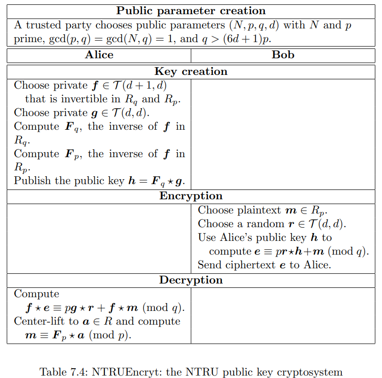
Encrypt

NTRU密码系统的加密

def encrypt(message,publickey):
    r = randomdpoly()
    return balancedmod(convolution(publickey,r) + message,q)

Decrypt

NTRU密码系统的解密

def decrypt(ciphertext,secretkey):
    f, f3 = secretkey
    a = balancedmod(convolution(ciphertext,f),q)
    return balancedmod(convolution(a,f3),3)

加密解密的原理比较简单，这里就不再赘述，但是要注意如果参数大于了正常的解密范围，极有可能引起解密失败，但可以通过标准化 $q,n,d$ 来解决， $q$ 的选取越小越好，因为多项式的系数可以为 {-1,0,1}这类

Attack

这里的攻击方式显然并不是恢复 $publickey$ 中的 $f(x)$ ，毕竟这也太靠脸了

由于NTRU的解密合法性，我们发现如果我们能找到一组 $f(x)$ 与 $g(x)$ 也满足 $key$ 的关系，那么我们就能拿这组多项式来充当新的 $key$

我们的矩阵构造如下
$$
B^{NTRU}
=
{\begin{bmatrix}
\pmb{1}&\pmb{h(x)} \\
\pmb{0}&\pmb{q}
\end{bmatrix}}
=
\begin{bmatrix}
\begin{array}{lllll|lllll}
1&0&0&\cdots&0&h_0&h_1&h_2&\cdots&h_{n-1} \\
0&1&0&\cdots&0&h_{n-1}&h_0&h_1&\cdots&h_{n-2} \\
0&0&1&\cdots&0&h_{n-2}&h_{n-1}&h_0&\cdots&h_{n-3} \\
\vdots&\vdots&\vdots&\ddots&\vdots&\vdots&\vdots&\vdots&\ddots&\vdots \\
0&0&0&\cdots&1&h_1&h_2&h_3&\cdots&h_0 \\
\hline
0&0&0&\cdots&0&q&0&\cdots&0 \\
0&0&0&\cdots&0&0&q&0&\cdots&0 \\
0&0&0&\cdots&0&0&0&q&\cdots&0 \\
\vdots&\vdots&\vdots&\ddots&\vdots&\vdots&\vdots&\vdots&\ddots&\vdots \\
0&0&0&\cdots&0&0&0&0&\cdots&q \\
\end{array}
\end{bmatrix}
$$
当然左上角也可以选任意的正整数 $\lambda$ ， 同余方程里 $f(x)$ 乘个系数 $\lambda$ 罢了，对 $B^{NTRU}$ 格基规约后得到的第一个向量就可以作为新的 $f’(x)$ 和 $g’(x)$ 了

据说可以添加一个大整数 $\theta$ ，这样方便规约，如下
$$
B^{NTRU}_{\theta}
=
{\begin{bmatrix}
\pmb{1}&\pmb{\theta h(x)} \\
\pmb{0}&\pmb{q\theta}
\end{bmatrix}}
$$
不过现在遇到的题基本上都是给的多项式计算后的数，直接用多项式的好像很少（？，但原理层面上是差不多的，只不过关系好推一点，代码实现起来也简单点吧

LWE (learning with error)

Waiting for undate……